I am really proud to be a co-author on a recent paper in npj Quantum Information. A lot of people worked on this paper — you can see the author list in the article. It is the product of ideas that I was discussing with Jasmin Meinecke and Nicolas Brunner over 5 years ago. Through relentless persistence of Jasmin and others, the result has at long last been published — no thanks to me!

Result

We describe a scheme to detect and classify quantum entanglement, even when the observers’ view of the quantum state in question is obscured by a dynamic, poorly-characterized, noisy environment.

This is cool to me because people often talk about entanglement as something that is “fragile”. In this paper, we show that you can put an entangled state through a really noisy environment — something that experimentalists might expect to kill the state — and the signal of entanglement is still just as strong as it was before.

Scenario

We consider a scenario which starts with an uncharacterized source of multipartite quantum states — a box which spits out $N$ qubits in a state $\hat{\rho}$. Under normal circumstances, if we wanted to understand the structure and quantity of entanglement in $\hat{\rho}$, we would do state tomography — a very standard sequence of specific measurements on consecutive copies of the state, from which we can learn everything that there is to know about $\hat{\rho}$.

State tomography is just like the procedure that you go through to build a mental model of a novel 3D object. You look at the object from some perspective, then you rotate it in your hands, take another image, rotate, take another image, and so on, and in doing so you can completely learn the geometry of the object in question. Tomography is the “T” in a CAT scan, which works the same way.

However, in this paper we up the ante in a way that makes tomography impossible:

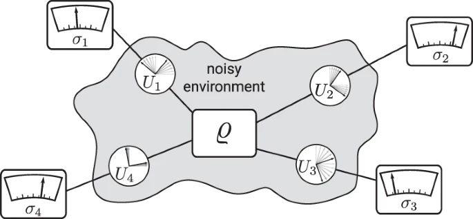
See that $\hat{\rho}$ in the middle there? It is now completely surrounded by a spooky grey cloud.
The cloud represents a real-world problem that frequently frustrates experimentalists. Each part of the quantum state is now getting distorted by an unknown, time-varying rotation that drifts in some unpredictable way.

This happens in real experiments when, for example, badly routed optical fiber gets bent and squashed, and thus causes random, fluctuating polarization rotations on photonic qubits. Magnetic field fluctuations can cause similar uncontrolled local rotations for trapped ions.

If you were to try to do tomography in this scenario, by the time you completed your first measurement, the fiber will have wriggled around a bit, and so your second measurement is potentially totally uncorrelated with the first — meaning that your final reconstruction of the state will be nonsense, and will not reveal any appreciable structure or entanglement.

There is a subtlety here. We assume that the drift in these uncontrolled rotations is fast enough that tomography is not possible, but slow enough that it is possible to acquire a few measurements before the rotation changes significantly.

Specifically, we assume that the rotations can be approximated to be unitary on the timescale of estimating an expectation value, but are uniformly (Haar) random on the timescale of evaluating multiple expectation values. If you want more details on this part, they are there in the paper. Basically, this captures the notion of “annoyingly fast drift” as opposed to full-on broadband noise.

Fast drift is enough to turn your carefully prepared, beautifully entangled quantum state into an unintelligible mess. Does the environmental noise irrevocably “destroy” the entanglement? No — entanglement is “invariant under local unitaries”. So every time we measure the state, we are potentially still dealing with a maximally entangled state — just one that has been spun about in some random fashion.

Scheme

So, what can we do in this scenario? Each of our measuring devices is perfectly calibrated, and can precisely measure in a whole range of different measurement “bases” — projecting the state in different directions on demand. However, that’s all a bit futile given that right before the state enters our measuring device, it is getting twisted up in some random and unknown way. What’s the point in measuring in a given direction, given that totally random rotations are happening anyway?

There’s no point — so let’s just always “measure in $\hat{Z}$”, i.e. project the state onto the $|0\rangle, |1\rangle$ basis. We’ll never bother changing the settings on our measurement device. Much easier than tomography with all those complicated different settings.

Formally, we are going to get expectation values of the form

$$ E(t) = \text{Tr}\left[ \hat{\rho} \hat{M}(t) \right] $$

where

$$ \hat{M}(t) = \bigotimes_i^N U_{i}(t)^\dagger \hat{\sigma}_z U_{i}(t) $$

is the $N$-qubit measurement operator modelling the product of the environmental rotation $U_i(t)$ at time $t$ and the action of our measuring apparatus, which is always $\hat{\sigma_z}$.

Given the constrained setting, the only option that is really available to learn about $\hat{\rho}$ is to take multiple measurements of $E(t)$ and look at the statistics.

$E(t)$ can take values in the interval $[-1, 1]$, and if the fluctuations $U_i(t)$ are uniformly random, the distribution of $E(t)$ in that interval will be symmetric about zero. Therefore, in the limit of many repeated measurements, the mean value of $E(t)$ will always be zero — the mean teaches us nothing.

That’s disappointing, but hardly surprising — we looked at the mean value of a symmetric random signal and found nothing. What can we do instead? Well, we could look at the moments. Whats the dumbest way to do that? How about take the absolute value of $E(t)$, to “reflect” the x-axis onto the interval $[0, 1]$? Sounds good, and using abs instead of the square is a great way to annoy mathematicians.

Distinguishing entangled states from product states

Now we have defined a repulsive new “observable”, $abs(E(t))$, which will move around in the interval $[0, 1]$ as the environment drifts.

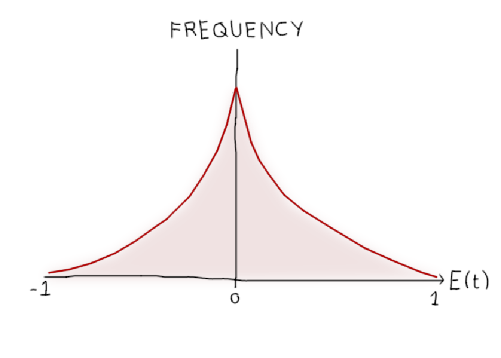
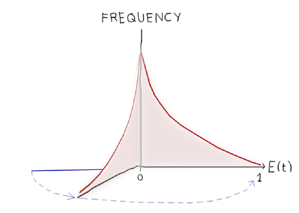
Let’s look at how this value is distributed for a product state (a state with no entanglement) versus a Bell state (the canonical maximally entangled two-qubit state).

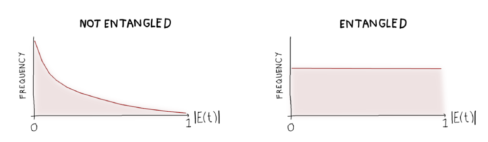
Ah, these look pretty different! If we just look at the average value of $abs(E(t))$ over time, we can very easily spot the difference between any product state and any maximally entangled state. In fact:

• For a product state, $\langle abs(E(t))\rangle = \frac{1}{4}$
• For a Bell state, $\langle abs(E(t))\rangle = \frac{1}{2}$

Putting that another way, the average of the absolute expectation value over all possible random local measurements is 1/4 for any product state, and 1/2 maximally entangled two-qubit state.

Further results

Telling the difference between Bell states and product states is nice, but in reality there are a lot more interesting states out there — mixed states, partially entangled pure states, and multi-qubit states with all sorts of interesting entanglement properties. It turns out that by looking at the statistics of the observable as described above, you can distinguish a wide diversity of different entanglement classes, and to some extent you can quantify the entanglement and purity of the state you are dealing with.

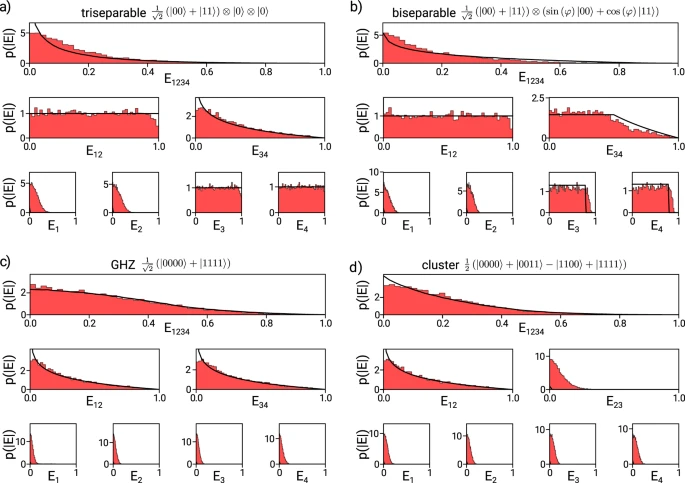
The figure above is real experimental data, showing the distributions that are generated for different types of entangled state. We are able to distinguish all the different classes of four-qubit state, including GHZ states:

Implications

For lazy experimentalists, the upshot is that you don’t have to compensate for slow-enough fluctuations, or calibrate your measuring gear, as long as all you want to learn is the structure of entanglement in your state. That means you never have to touch one of these:

In principle you could learn if a two-photon state is entangled or not just by shaking the fiber around like crazy. We actually tried this in the lab, and it works.

What if the environmental noise isn’t Haar-random?

The measuring apparatus itself is well under control. If the drift is not uniform, you can just make sure to measure in a different Haar-random basis each time you evaluate an expectation value.